We estimate your admission chances by rebuilding the admissions cycle itself: a full cohort of simulated students competes for real seat counts at 200 colleges across six rounds — and we run that cycle hundreds of times. Every input comes from published institutional data, and we end with the calibration receipts so you can check our work.
Some systems have too many moving parts to solve with a single formula. In the 1940s the mathematician Stanisław Ulam realized that instead of solving the equations, you could build a working model, run it over and over with the randomness left in, and simply count the outcomes. His colleague Nicholas Metropolis named it after the Monte Carlo casino — fitting, because at heart it's repeated dice-rolling, done seriously, at scale. You already rely on it: "70% chance of rain" means forecasters ran the atmosphere forward many times and it rained in 70% of them.
Admission is exactly that kind of system — it depends on your profile, but also on who else applies, in which rounds, and how each college manages its yield. So we simulate a whole admissions cycle, from Early Decision through waitlists, and run it hundreds of times. Admitted in 160 of 500 cycles? Your chance is 32%. And because every decision in a cycle happens to the same simulated you, the model captures how your outcomes correlate across your list — letting it estimate real risks like striking out everywhere, which eight isolated percentages can't.
Why simulate instead of fitting a formula?
Most chancing tools fit a regression to past data: GPA + SAT + extracurriculars in, a percentage out. That ignores the thing that actually decides who gets in — which other students are competing for the same seats. Admission isn't a score you clear; it's a competition against a specific pool. So we model the pool. Each simulated student is an agent with their own academics, hooks, high-school context, and college list, sampled so the population matches what admissions offices actually see. A college with 1,500 seats and 50,000 applicants admits from the top; your chance is how often you make the cut.
200
Colleges modeled
17,884
High schools
6
Admission rounds
500+
Cycles simulated
Your high school matters more than people expect: the same GPA means different things at different schools, and colleges read applications in context. When you tell us where you go, the simulation builds your competitive environment around it — drawing on 17,884 US high schools — instead of dropping you into a generic national average.
Which admission factors does the model weigh?
The factor set comes from the Common Data Set colleges publish each year. Section C7 states which factors each treats as very important, important, considered, or not considered — and the model weighs what each says matters:
Academic strength — unweighted GPA, SAT/ACT, and course rigor, measured against the college's own middle-50% ranges, not a national average.
Hooks — legacy, recruited athlete, development case, and first-generation, each weighted from peer-reviewed research and per-college disclosures.
Round and pool effects — Early Decision gives a real boost; a deep Regular pool is harder. Both are modeled separately, along with per-college demonstrated interest where the CDS says it's considered.
How does the scoring work?
Every applicant–college pair gets one admission score. The factor families above are combined additively in logit space (log-odds), then passed through a sigmoid to produce a probability between 0 and 1:
Working in logit space means a hook or an early round shifts your odds by a consistent factor rather than a fixed number of points — worth a lot at a 40%-admit college, proportionally less at a 4%-admit one, which is how real preferences behave. The per-college constant anchors the score to that college's actual selectivity. Admission is then a random draw against P(admit) each cycle, so competition for limited seats plays out agent by agent, round by round.
The exact form, weights, and per-college constants are proprietary — but how we ground them isn't: every weight is anchored to a published source or peer-reviewed study, and every per-college constant is calibrated against that college's most recent Common Data Set. Two structural details matter: international students compete for a separate slice of seats per college (from ~1% at big publics to a quarter of the class at the most international-heavy privates), so they don't crowd the domestic pool; and each cohort is a representative sample of who actually applies to each school, not just the visible agents.
How are early and regular rounds modeled?
Real admissions is sequential; the engine runs the same sequence, where most tools collapse it into a single rate. ED commits you to one school, EA leaves options open, deferrals roll forward, and melt happens after May 1.
Round 1
Early Decision (ED)
Binding. A substantial admit-rate advantage in exchange for commitment — at many selective private colleges, binding early rounds fill 40–60% of the incoming class.
Round 2
Early Action / REA
Non-binding early. Smaller boost than ED but no commitment trade-off. Top-tier schools that don't offer ED concentrate here.
Round 3
Early Decision II
Second binding round in January. Used by students whose ED1 was rejected or by late deciders.
Round 4
Regular Decision (RD)
The bulk of applications. Largest pool, hardest acceptance rate.
Round 5
Student decisions & melt
Admitted students choose where to enroll based on a yield model (preference + cost + fit). Some students "melt" — accept, then withdraw before fall.
Round 6
Waitlist activation
If a college misses its yield target after melt, it activates the waitlist to fill remaining seats.
Most chancing tools ask you to take their numbers on faith. We publish the receipts. Below, every one of the 192 colleges is one dot — x-axis its published Common Data Set acceptance rate, y-axis the rate our simulation produced by running the personalized engine across a nationally-representative applicant sample (every school type and feeder tier, in realistic proportion) and pooling the result. The dashed line is perfect agreement (y = x); the solid green line is the proportional best fit.
Simulated vs. published acceptance rate
All 192 colleges, personalized engine, pooled across a nationally-representative applicant sample. Hover any point for details. The stats below are computed live from the shipped calibration file.
Points hug the diagonal — a college twice as selective in CDS data is roughly twice as selective in our simulation — with a Pearson r of 0.98 and a mean ratio near 1.0×, meaning the model tracks real acceptance rates with no systematic bias in either direction. The tightest agreement is at the selective end that most applicants are weighing (Stanford lands near Yale, not near a state flagship); the widest spread is among a handful of large public universities, where in-state versus out-of-state dynamics make a single "overall" rate a blunt yardstick. Above all, the model reproduces relative selectivity — how your odds compare across your list — which is the question that should actually drive where you apply.
Precision: why hundreds of cycles
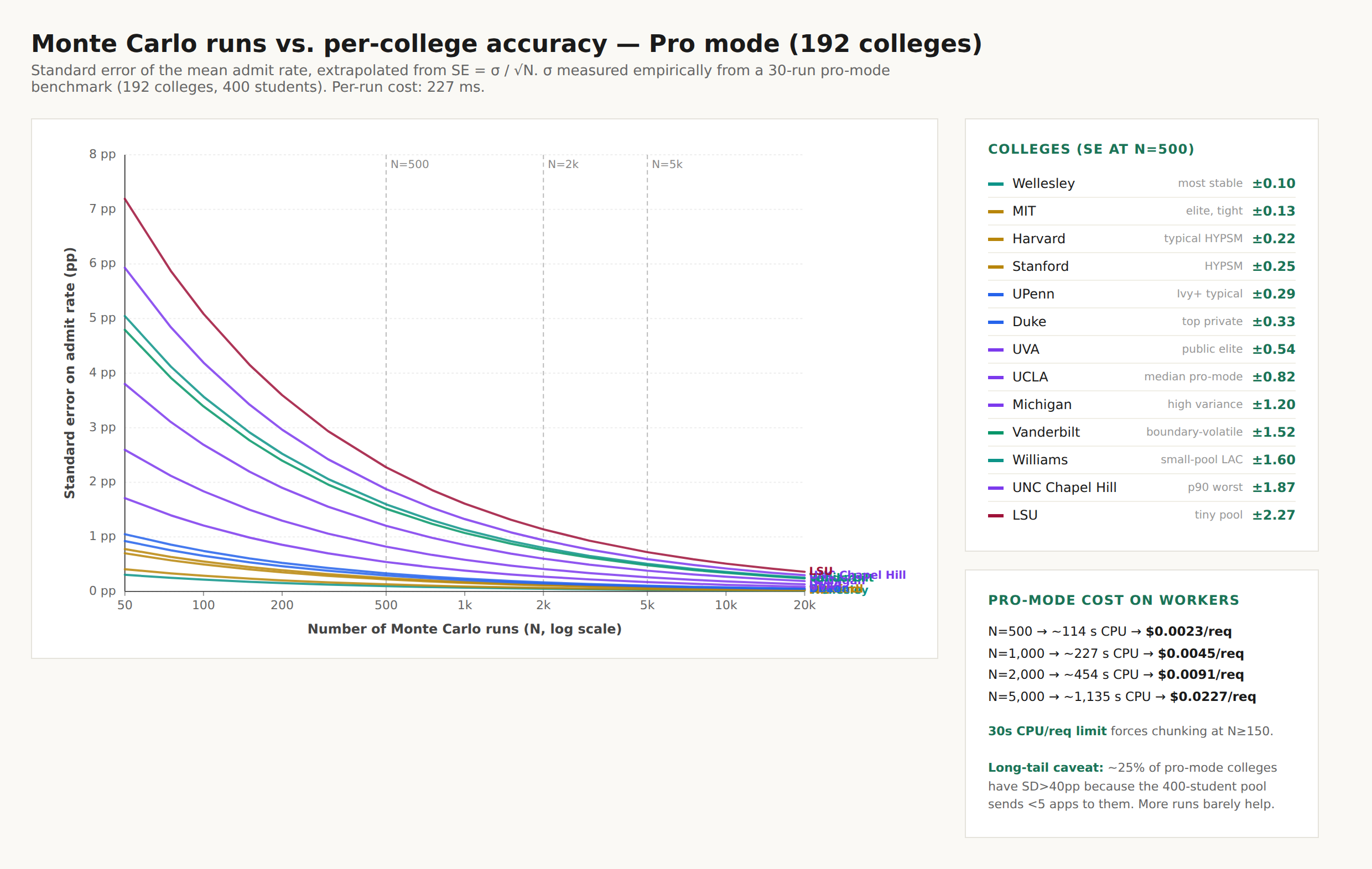
Accuracy is whether the dartboard is in the right place; precision is how tight the grouping is. Monte Carlo error shrinks predictably with more runs, so our tools put each profile through 500 to 800 cycles — past the elbow where per-college standard error has fallen from a few points to about one.
Alongside admission odds, the tools show an estimated net cost at each college. Cost never touches the admission decision — it's a separate layer. The anchor is IPEDS net-price data by household income bracket: what students from families like yours actually paid after grants and scholarships, for the 2025–2026 award year. The cost engine then refines that per family — computing your FAFSA Student Aid Index from income, assets, home equity, and family size, and overlaying CSS Profile conventions for meets-full-need private colleges. See paying for college: understanding net price.
Where does the data come from?
Every input is public institutional data, not anecdote, updated against current cycles each year:
Common Data Set (2024–2025). Per-college acceptance rates, SAT percentiles, yield, ED/EA breakdown, class size, demographics — each college publishes its own; it's the gold standard.
NCES surveys + state DOE files. The backbone of 17,884 US high schools, blended with 12 state departments that publish school-level SAT/ACT means.
IPEDS and the College Scorecard. Net price by income bracket, degree completions, and graduate earnings — used in the chancing and cost UIs, never in the admission decision.
Published research. Hook effects from peer-reviewed work on legacy and athletic preferences (Arcidiacono et al.; Hurwitz); early-round yield behavior from Avery & Hoxby. Full bibliography in Research.
A 20% chance means you got in in roughly one of five simulated cycles — not that you'll be rejected. Estimates depend on the full profile: holistic inputs like essay quality and extracurricular depth are self-assessed, and no model sees your actual essays or recommendations.
What the calibration supports is relative selectivity — how your odds compare across colleges. Treat any single percentage as a planning input, not a prediction about you personally.
Further reading:
Data Sources — provenance for every metric in the product.